Lesson 2.2: Tidying and merging data

Lesson 2.2: Tidying and merging data#

As of now, our data for water temperature for Stream A and B exists in a separate data frame from the dissolved oxygen concentrations for Stream A and B. For K’avi Fish and Wildlife managers to truly understand what’s going on, they need to analyze water temperature and dissolved oxygen together. To do this, we need to change how our data is set up in each data frame and then merge these data frames together.

Manipulating data so that it is formatted in a way that we can easily and reliably analyze is called “data wrangling”. In R, we like our data to be “tidy”. This means we don’t want duplicate columns for the same variable. For example, in the stream_temp dataset, we have two columns for temperature, because we have a column for the water temperature of Stream A and the water temperature of Stream B. In a “tidy” version of thus dataset, we want all the temperature values to be in the same column.

visual explainer of tidy data

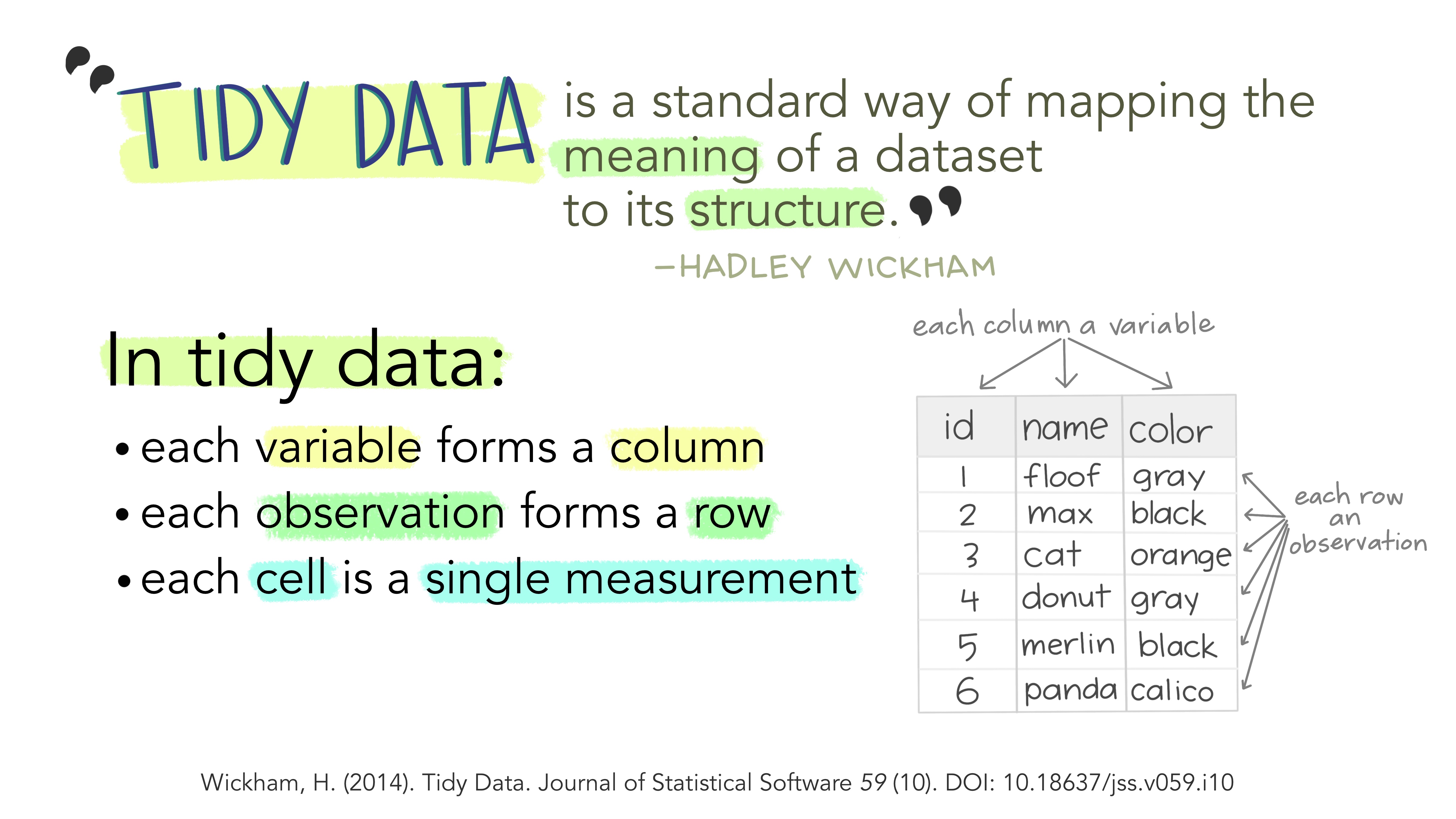
To learn more about tidy data, here’s a useful website.

# Load packages 
if(!require("tidyverse")) install.packages("tidyverse")
library(tidyverse)

# if running in google colab, uncomment and use the following lines:
# stream_temp <- read.csv("https://raw.githubusercontent.com/rachtorr/IndigenousEnvDataSci.github.io/refs/heads/main/MOD2/streams_temperature.csv")
# stream_DO <- read.csv("https://raw.githubusercontent.com/rachtorr/IndigenousEnvDataSci.github.io/refs/heads/main/MOD2/streams_DissolvedOxygen.csv")

# read in stream temp data 
stream_temp <- read.csv("streams_temperature.csv", header=TRUE, sep=",")
# read in dissolved oxygen data 
stream_DO <- read.csv("streams_DissolvedOxygen.csv", header=TRUE, sep=",")

Error in library(tidyverse): there is no package called ‘tidyverse’
Traceback:

1. stop(packageNotFoundError(package, lib.loc, sys.call()))

Tidying data#

First, we will use the pivot_longer() function to reorganize the columns from the temperature dataset, so that there is one column for “site” and one column for “temperature_C” The goal is to make only one column for each variable.

Look back at the current “messy” version of stream_temp. Can you see that there is more than one column with the same variable?

The pivot_longer() function allows us to combine columns, which transforms our dataset into a form with more rows (longer), and fewer columns (less wide). Long form data makes it easier to summarize data and look at trends over time, which allows the tidyverse package to work better.

In the code chunk below, we use pivot_longer() to transform the temperature data. The #comments describe what each line of code does. We rename our data frame and then preview it with head().

# The first line of code tells R that we want to re-define 
# the streams_temp dataset with the changes we make below. 
# This weird thing %>% is called the "pipe". It says that the code lines that come next, 
# which are linked by a "+" at the end of each line,
# will all contribute to a transfomed version of stream_temp. 

stream_temp_long <- stream_temp %>%  
# We use the pivot_longer code to tell R which columns we want to change.
  pivot_longer( 
    #cols = tells R which columns we want to modify
    cols = c(StreamA, StreamB), 
    # names_to tells R that we want the names of the columns we specified 
    # above to be entries in a new column we're creating called "site". 
    names_to = "site", 
    # Question: Based on what "names_to" means, what do you think the next line 
    # of code values_to means? 
    # (Hint - searching the internet for the answer is a great way to figure this out.)
    # Looking things up online is a huge part of coding!
    values_to = "temperature_C" 
  )

head(stream_temp_long)

A tibble: 6 × 3
year	site	temperature_C
<int>	<chr>	<dbl>
2007	StreamA	13.2
2007	StreamB	10.2
2008	StreamA	12.5
2008	StreamB	NA
2009	StreamA	13.9
2009	StreamB	NA

Great! Our code worked. Now let’s do the same for the dissolved oxygen data set.We want to change it in the same way we changed the temperature data set above.

💻 HOWEVER, this time some chunks of code have been left blank. See if you can fill them in based on what you saw in the example above!

stream_DO_long <- stream_DO %>%  
# We use the pivot_longer code to tell R which columns we want to change.
  pivot_longer( 
    # [FILL THIS IN]
    cols = c(), 
    # names_to tells R that we want the names of the columns we specified 
    # above to be entries in a new column we're creating called "site". 
    names_to = "site", 
    values_to = "dissolved_oxygen" 
  )

Again, we should check our work to make sure that our data looks the way we want it to. We want there to be three columns, one for the year the sample was collected, one for the site name, and one for the dissolved oxygen values (mg/L).

print(stream_DO_long)

# A tibble: 32 × 3
    year site    dissolved_oxygen
   <int> <chr>              <dbl>
2007 StreamA             7.18
2007 StreamB            NA   
2008 StreamA             7.27
2008 StreamB             8.07
2009 StreamA             7.46
2009 StreamB             7.26
2010 StreamA             7   
2010 StreamB            NA   
2011 StreamA             6.53
2011 StreamB            NA   
# ℹ 22 more rows

The data frame is now in a ‘tidy’ format because it has a single observation per row, with one column of the ‘site’ and one of the ‘dissolved oxygen’ that contains the observation values.

Merging data frames#

So far, we have separate dataframes for temperature and DO. We want to combine them into one tidy dataframe, so we can analyze trends in temperature and dissolved oxygen at the same time for both streams.

To do this, we will use a command in tidyverse called full_join(), from the join commands. Full join means we want to combine two data frames. We want to match up the rows in the first data frame with the second data frame based on a matching key that the two have in common - in our case the year and site. See more on the join commands here.

The format for joining is: full_join(dataframe1, dataframe2, by=c(columns they have in common))

# Here, we are using full_join to put the streams_temp data frame next to the streams_DO data frame.
streams_joined <- full_join(stream_temp_long, stream_DO_long, by=c("year","site"))

# preview what our new data frame looks like 
head(streams_joined)

A tibble: 6 × 4
year	site	temperature_C	dissolved_oxygen
<int>	<chr>	<dbl>	<dbl>
2007	StreamA	13.2	7.18
2007	StreamB	10.2	NA
2008	StreamA	12.5	7.27
2008	StreamB	NA	8.07
2009	StreamA	13.9	7.46
2009	StreamB	NA	7.26

Great job data wrangling! We now have a single tidy dataframe that we can use to analyze water quality and determine which stream is best for introducing bull trout to tribal land.

Now that we have a data frame in the format we want, it’s good practice to save the dataframe so that you don’t need to repeat the steps from above. We will do this using the write.csv() function, which takes two main inputs: the data frame we are saving, and the file name with location.

# save our tidy data frame 
write.csv(streams_joined, "streams_data.csv")

Lesson 2.2 Recap:#

In this lesson we have learned the following:

wrangling data into a tidy format, with one observation per row
using pivot_longer() to reduce multiple columns into two columns with a key and a value. In our case, the stream ID was the key, and the observation was the temperature or DO value
merging two data frames using full_join(), which combines dataframes using identifying columns that both data frames have in common - in our case, year and site

Lesson 2.2: Tidying and merging data

Contents

Lesson 2.2: Tidying and merging data#

Tidying data#

Merging data frames#

Lesson 2.2 Recap:#